Model design
Spatial econometric model
DI and regional GIE have strong spatial correlation (Hu et al. 2023; Song et al. 2018; Li and Du, 2021). Should this study neglect this inherent spatial spillover effect, it would produce biased empirical result. Hence, the model employs a spatial panel model. Spatial econometric models are valuable tools for analyzing spatial spillovers, and primarily include the spatial autoregressive model (SAR), the spatial autocorrelation model (SAC), the spatial error model (SEM), and the SDM (LeSage and Pace, 2009; Anselin, 2013). Spatial correlations may arise from the dependent variable, the explanatory variable, or the error term. The SDM effectively captures the spatial correlation from various sources (Elhorst, 2014). LeSage and Pace (2009) conduct a comparison of the four models above, assuming that the original data adhered to the data generation process of SAR, SEM, SDM, and SAC, respectively. The authors examine the estimation results that may have been caused by potential model errors, determining that the SDM model is the only model that can obtain unbiased estimations. According to the purpose of this study and the hypotheses in Section “Theoretical analysis”, this study constructs the following SDM panel approach:
$$\begin{array}{l}GI{E}_{it}=\alpha +\varphi \mathop{\sum }\limits_{j=1}^{n}{w}_{ij}GI{E}_{jt}+\beta D{I}_{it}+\rho \mathop{\sum }\limits_{j=1}^{n}{w}_{ij}D{I}_{jt}+\gamma {X}_{it}\\\qquad\qquad+\,\theta \mathop{\sum }\limits_{j=1}^{n}{w}_{ij}{X}_{jt}+{\mu }_{i}+{\lambda }_{t}+{\varepsilon }_{it}\end{array}$$
(1)
$${\varepsilon }_{it}=\varphi \mathop{\sum }\limits_{j=1}^{n}{w}_{ij}{\varepsilon }_{it}+{\mu }_{it},\mu \sim N(0,{\sigma }_{it}^{2})$$
(2)
where GIE denotes the regional GIE, DI represents the regional DI index, X represents control variables, α is a constant term, ε is a random error, i represents the prefecture-level region, t pertains to the year, μi and λt refer to regional and time fixed effects, wij denotes a spatial weight matrix, φ is the spatial regression coefficient. β, ρ, γ and θ are the coefficient to be estimated.
Selection of spatial distance matrix
A spatial weight matrix is used to quantify the spatial adjacency of locations to reveal spatial interaction effects. Constructing a suitable spatial weight matrix can describe the degree of correlation between spatial units. Due to the large number of prefecture-level cities in China, simply determining whether the cities are adjacent may result in a loss of valuable information. There may be deviations in measuring the spatial correlations between regions by any distance standard (geographical distance, economic distance). Therefore, referencing Parent and LeSage (2008), this study adopts the nested matrix of geographical and economic distance (WW), which considers the spatial impact of geographical distance and simultaneously reflects the regional spillover and radiation effects of economic factors. This spatial weight matrix reflects the spatial correlation degree between regions more comprehensively and objectively, and its specific form is as follow:
$$Ww=\varphi Wd+(1-\varphi )We$$
(3)
$$Wd=\frac{1}{{d}_{ij}^{2}},We=\frac{1}{|{g}_{j}-{g}_{i}|}$$
(4)
where Wd is the reciprocal square of the distance between the longitude and latitude of regions i and j, and We represents the reciprocal of the absolute value of the difference in per capita GDP between regions i and j. This φ value is set at 0.5.
Mediating effect model
To investigate the transmission mechanisms of potential mediating variables on the impact of DI on regional GIE, referencing Dell (2010), this study employs the following two-step method to establish a mediating effect model:
$$\begin{array}{l}{l}Mec{h}_{it}={\alpha }_{1}+{\varphi }_{1}\mathop{\sum }\limits_{j=1}^{n}{w}_{ij}Mec{h}_{jt}+{\beta }_{1}D{I}_{it}+{\rho }_{1}\mathop{\sum }\limits_{j=1}^{n}{w}_{ij}D{I}_{jt}\\\qquad\qquad+\,{\gamma }_{1}{X}_{it}+{\theta }_{1}\mathop{\sum }\limits_{j=1}^{n}{w}_{ij}{X}_{jt}+{\mu }_{i}+{\lambda }_{t}+{\varepsilon }_{it}\end{array}$$
(5)
where \(Mec{h}_{i,t}\) represents a series of intermediate variables, and other symbols are consistent with Eq. (1).
Variable interpretation
Dependent variable
Regional GIE is the explanatory variable of this study. According to the assumption of constant return to scale, referencing Wang et al. (2022), this study uses the undesirable super-efficiency EBM model to assess regional GIE. The undesirable super-efficiency EBM model is constructed as follows:
$$\rho =\,\min \frac{\phi -{\varepsilon }^{-}{\sum }_{m=1}^{M}{w}_{m}^{-}{s}_{m}^{-}/{x}_{k,m}}{\theta +{\varepsilon }^{+}({\sum }_{j=1}^{J}{w}_{j}^{+}{s}_{j}^{+}/{y}_{k,j}+{\sum }_{p=1}^{p}{w}_{p}^{u-}{s}_{p}^{u-}/{u}_{k,p})}$$
(6)
$$s.t.\left\{\begin{array}{c}\begin{array}{c}\mathop{\sum }\limits_{n=1,n\ne k}^{N}{x}_{n,m}^{t}{\lambda }_{n}^{t}+{s}_{m}^{-}\le \phi {x}_{k,m}\\ \mathop{\sum }\limits_{n=1,n\ne k}^{N}{y}_{n,j}^{t}{\lambda }_{n}^{t}+{s}_{j}^{-}\le \theta {y}_{k,j}\\ \mathop{\sum }\limits_{n=1,n\ne k}^{N}{u}_{n,p}^{t}{\lambda }_{n}^{t}+{s}_{p}^{-}\le \theta {u}_{k,p}\end{array}\\ \lambda \ge 0,{s}_{m}^{-}\ge 0,{s}_{p}^{+}\ge 0\end{array}\right.$$
(7)
where ρ refers to the GIE of the area being assessed; \({x}_{m}\), \({y}_{j}\), and \({u}_{p}\) denote the input, desirable output and undesirable output, respectively; \({w}_{m}^{-}\), \({w}_{j}^{+}\), and \({w}_{p}^{u-}\) denote the weights of the input, desirable output, and undesirable output, respectively; \({s}_{m}^{-}\), \({s}_{j}^{+}\), and \({s}_{p}^{u-}\) denote the slacks of the input, expected output, and unexpected output, respectively. Parameters ϕ and θ denote the radial components. Additionally, ε is a key parameter reflecting the combination of radial and nonradial relaxation, and its value is between 0 and 1. When ε’s value is 0, the model is equivalent to the radial model, and when its value is 1, the model will degenerate into a nonradial SBM model. Considering data availability, the input and output variables for calculating regional GIE are defined as follows:
The input variable includes labor, capital, and energy, which are measured by the total number of regional R&D personnel (people), internal regional R&D expenditure (10,000 yuan), and regional power consumption (10,000 kwh), respectively. Expected output includes economic, green technology innovation, and ecological income outputs, which are measured by actual urban GDP (10,000 yuan), the number of regional GI patent applications (pieces), and the green space coverage rate of urban built-up areas (%), respectively. Actual urban GDP is measured by the constant price in 2013. For unexpected output, this study uses the entropy weight method to calculate the comprehensive pollutant emissions index, which is respectively expressed by the emissions of urban industrial wastewater (tons), urban industrial waste gas (tons), and urban solid waste (tons). To ensure that the conclusions are robust and credible, the robustness test uses the ratio of total number of green invention patent applications and urban government scientific research expenditure to construct replacement indicators.
Core explanatory variables
DI is the core explanatory variable of this study. Some controversies concerning the measurement of DI still remain in existing studies, and the Broadband China policy pilot is predominantly used as an indicator to measure DI (Ma and Lin, 2023). However, DI is a comprehensive, multidimensional concept. In view of this, referencing Tang and Yang (2023), this study constructs a comprehensive DI index, using three dimensions of information development (measured by optical cable and mobile phone base station density), internet development indicators (measured by traditional internet penetration, mobile internet penetration, the number of internet broadband access ports, and number of IPv4 addresses), and digital transaction development indicators (measured by the number of websites per 100 enterprises). These measures are then integrated into the comprehensive DI index using an entropy weight method. Due to data limitations in the China Urban Statistical Yearbook, the majority of previous research uses indicators such as the number of internet users per capita and the volume of post and telecommunications services as proxy variables to measure DI at the urban level. Although these are directly related to cities’ supply of DI, they are more affected by consumers’ communication demand. In contrast, this study uses the above indicators to build a comprehensive DI index to quantify DI at the city level to identify the impact of exogenous changes in the supply of urban DI on the efficiency of regional GIE more accurately. Because the supply side DI data are only reported at the provincial level, this study references Bartik (1991), calculating the weight index of the number of urban internet users as an exogenous weight, and decomposing the level of DI at the provincial level to the urban level as follows:
$$D{I}_{it}=weigh{t}_{ij}infra{s}_{pt}$$
(8)
where weight is the proportion of the number of internet users in each city in the province, and \(infra{s}_{pt}\) is the DI index in each province.
Control variables
To accurately capture the net impact of DI on regional GIE, this study introduces the following series of control variables into the regression model based on relevant research.
Human resources (HR)
Education provides the HR required for advancing national innovation, and regions with high HR are able to attract high-tech enterprises (Zhang et al. 2020). This variable is measured by the number of students in colleges and universities per million people.
Openness degree (OPEN)
The advanced production equipment, technology, and management experience of foreign enterprises have spillover effects, which may improve local GI efficiency; however, the pollution paradise hypothesis contends that excessive OPEN will inhibit GIE (Hao et al. 2023). This variable is measured by the ratio of total imports and exports to GDP.
Fiscal freedom (FF)
A higher degree of government FF indicates higher talent accumulation and capital investment, which can increase GIE (Lin and Ma, 2022). This variable is measured by the ratio of regional general public budget revenue to regional general public expenditure.
Industrial structure (IS)
Industrial structure differences can objectively reflect variations in resource endowment, input factors, and other conditions at the city level. This difference may generate different degrees of difficulty and choices for entrepreneurship in different cities, which will affect cities’ GIE (Zhang et al. 2023). This variable is measured by the proportion of the city’s added value by the secondary industry.
Population density (PD)
Overly high PD may produce increased environmental pollution, which reduces regional GIE. This variable is measured using the logarithm of urban per capita land use area.
Degree of economic development (GDP)
Economic growth may stimulate the improvement of GIE (Zeng et al. 2021; Dian et al. 2024). This variable is measured by the logarithm of per capita GDP.
Government support (GS)
GS for enterprise R&D funds and market economy intervention can mitigate the externalities of technological innovation activities and reduce the R&D risks associated with GI (Zhu et al. 2021). This variable is measured by the logarithm of government expenditure on science and education.
Data description
Given data availability and accessibility, this study uses balanced panel data of 281 prefecture-level cities in China from 2013 to 2020. This study obtains the patent grant data of GIE from the State Intellectual Property Office of China. The regional GDP index is from the China Statistical Yearbook (2013–2020). The DI indicators’ data are from the China Provincial Statistical Yearbook (2013–2020). Other indicators come from the city wide data in the statistical yearbook of Chinese cities (2013–2020). In addition, missing data for individual samples are obtained from the statistical yearbook of each prefecture-level city, statistical bulletins, official websites, the WIND database, or supplemented using interpolation. The descriptive statistics of all variables are presented in Table 1. As noted in the descriptions above, certain variables are transformed into natural logarithms to reduce heterogeneous randomness.
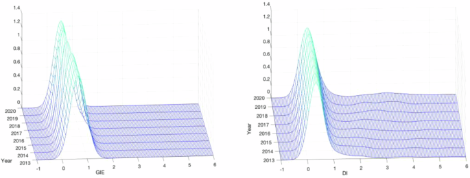
Using the nonparametric kernel density estimation equation and MATLAB software, this study determines the kernel density curve of China’s urban DI level and GI efficiency from 2013 to 2020 (Fig. 2). The nuclear density analysis can describe the dynamic evolution of China’s regional DI and GIE. Four notable findings emerge from this analysis. (1) From the position of the main peak, in terms of DI, the focus has been moving to the right from 2013 to 2020, indicating that regional DI in China increased during the study period. In terms of GIE, the focus shifted slightly to the right from 2013 to 2020, indicating regional GIE improvement. (2) Examining the shape of the main peak, the prominent peak of the curve exhibits a rising trend, revealing that the absolute differences in DI and GIE between regions are narrowing. This indicates that the height of the main peak continues to rise, and the width is gradually shrinking, showing that DI and GIE have improved to some extent. (3) From the perspective of distribution extensibility, a right tailing phenomenon is revealed in the construction of DI and GIE, revealing a gap within the region based on large regional development differences, including regions with high DI and regions with high GIE. Furthermore, the two distribution curve reveal a broadening convergence trend, indicating that although differences in regional DI and GIE are evident, the absolute difference has a narrowing trend. (4) From the perspective of polarization, no obvious polarization phenomenon in DI and GIE is apparent, with no gradient effect between them. DI construction is the core support for advancing regional digital and green development.

Dynamic evolution of DI and GIE (2013–2020).
link

